Supervised Learning Algorithms: Machine Learning Series for Beginners

Introduction

In our previous blog, we discussed data preprocessing, an essential step in preparing your dataset for machine learning. Now, we’ll focus on Supervised Learning Algorithms, one of the most popular types of machine learning techniques. Supervised learning involves using labeled data to train a model, making it capable of predicting outputs for unseen inputs.

This blog will cover the theory and practical implementation of three foundational algorithms:

1. Linear Regression
2. Logistic Regression
3. Decision Trees

We’ll provide Python code examples, explain key mathematical concepts, and discuss the strengths and weaknesses of each algorithm.

Figure 1: Supervised Learning Algorithm

Figure 1, provides a visual guide to selecting the appropriate Supervised Learning Algorithm based on the problem at hand. It compares Linear Regression for predicting continuous outcomes, Logistic Regression for binary classification problems, and Decision Trees for handling complex decision-making with multiple input features. The figure highlights the key strengths of each algorithm, helping users make informed choices in their machine learning projects.

1. What is Supervised Learning?

Detailed Explanation: Supervised learning uses input-output pairs (features and labels) to train models. The goal is to learn a mapping function f(X)→Y such that when given new inputs X, the model can predict the corresponding outputs Y.

There are two main types of supervised learning tasks:

1. Regression: Predicting continuous numerical values (e.g., house prices, temperature).
2. Classification: Predicting discrete categories (e.g., spam vs. not spam, disease vs. no disease).

Analogy: Think of supervised learning like a teacher grading a student’s answers. The student (the model) is shown questions (features) along with correct answers (labels) during training. Later, the student is tested on new questions to see how well they learned.

Figure 2: Regression and Classification

Figure 2, explains the concept of Supervised Learning by categorizing its two main tasks: Regression and Classification. Regression involves predicting continuous numerical values, such as house prices or temperatures, while classification focuses on predicting discrete categories, like spam or non-spam emails.

2. Key Supervised Learning Algorithms

2.1 Linear Regression

Purpose: Linear Regression predicts continuous outcomes by modeling a linear relationship between the input features and the target variable.

Example: Imagine you’re running a lemonade stand. You notice that as the temperature rises, more people buy lemonade. You keep track of the temperature and the number of glasses sold. By plotting this on a graph, you find that the relationship is roughly a straight line. Using this line, you can predict how many glasses of lemonade you’ll sell on a particularly hot day. That’s Linear Regression — finding a straight-line relationship between two variables to make predictions.

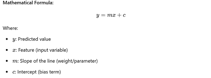
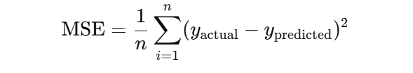
The model minimizes the Mean Squared Error (MSE) to find the best-fit line:

Python Implementation: Predict house prices based on square footage.

import pandas as pd
from sklearn.linear_model import LinearRegression
from sklearn.model_selection import train_test_split

# Create dataset
data = {'Square_Footage': [1500, 2000, 2500, 3000, 3500],
        'Price': [300000, 400000, 500000, 600000, 700000]}
df = pd.DataFrame(data)

# Split data into features and labels
X = df[['Square_Footage']]
y = df['Price']

# Train-test split
X_train, X_test, y_train, y_test = train_test_split(X, y, test_size=0.2, random_state=42)

# Train the model
model = LinearRegression()
model.fit(X_train, y_train)

# Predict
predictions = model.predict(X_test)
print("Predicted Prices:", predictions)

Strengths:

• Simple and interpretable.
• Works well for linear relationships.

Weaknesses:

• Sensitive to outliers.
• Fails to capture non-linear relationships.

Figure 3: Concept of Linear Regression

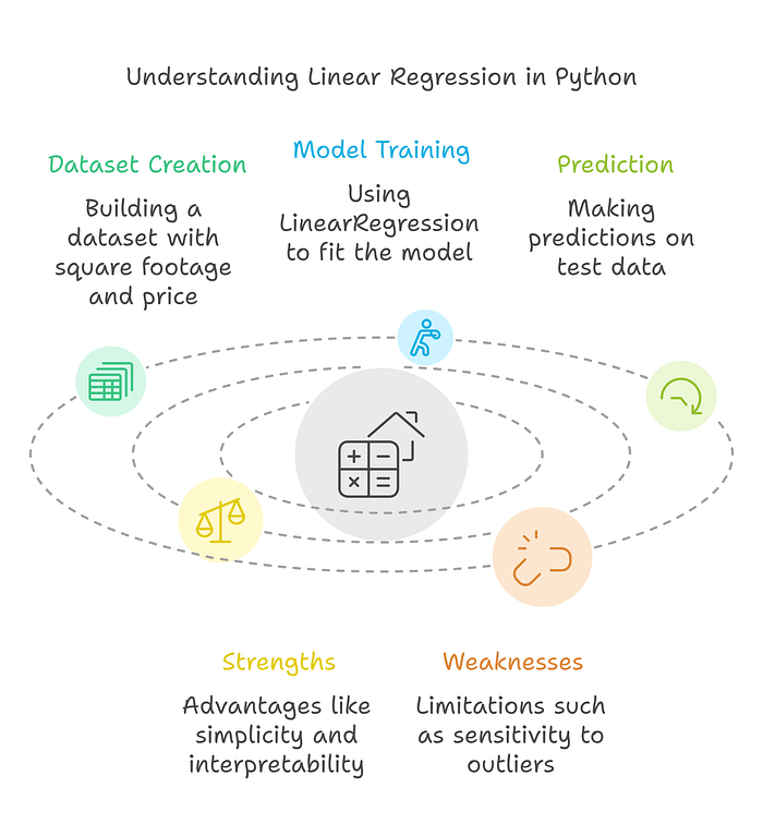
Figure 3, illustrates the concept of Linear Regression. It shows how a best-fit straight line is drawn through a scatter plot of data points, modeling the linear relationship between the independent variable (feature) and the dependent variable (target). The figure demonstrates how Linear Regression predicts continuous outcomes by minimizing the differences (errors) between the actual data points and the predicted values on the line, using the least squares method. This visual aids in understanding how Linear Regression works to make accurate predictions based on input features.

2.2 Logistic Regression

Purpose: Logistic Regression is a classification algorithm used to predict binary outcomes (e.g., 0 or 1, spam or not spam).

Example: Think of logistic regression like deciding whether to carry an umbrella. You check the weather forecast (input data), and based on the probability of rain (output probability), you make a binary decision: Yes (carry the umbrella) or No (leave it at home). Logistic Regression works similarly, predicting probabilities and then converting them into categories like rain or no rain.

Mathematical Foundation: Instead of a linear function, Logistic Regression uses the Sigmoid

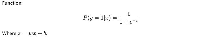
The sigmoid maps values to probabilities between 0 and 1, allowing for classification.

Python Implementation: Classify emails as spam or not spam based on word frequency.

from sklearn.linear_model import LogisticRegression

# Create dataset
data = {'Word_Frequency': [0.2, 0.8, 0.1, 0.4, 0.9],
        'Spam': [0, 1, 0, 0, 1]}
df = pd.DataFrame(data)

X = df[['Word_Frequency']]
y = df['Spam']

# Train-test split
X_train, X_test, y_train, y_test = train_test_split(X, y, test_size=0.2, random_state=42)

# Train the model
model = LogisticRegression()
model.fit(X_train, y_train)

# Predict
predictions = model.predict(X_test)
print("Predictions:", predictions)

Strengths:

• Probabilistic outputs.
• Works well for linearly separable data.

Weaknesses:

• Assumes linear decision boundary.
• Limited to binary classification (though it can be extended).

Figure 4: overview of Logistic Regression

Figure 4, provides an overview of Logistic Regression, highlighting its Python implementation, mathematical foundation, strengths, and weaknesses. It outlines the key steps for implementing Logistic Regression, including dataset creation, train-test split, model training, and prediction. The figure also explains the sigmoid function and probability mapping as the mathematical basis of the algorithm. It emphasizes the strengths of Logistic Regression, such as probabilistic outputs and suitability for linearly separable data, while also pointing out its limitations, like reliance on a linear decision boundary and restriction to binary classification.

2.3 Decision Trees

Purpose: Decision Trees classify data by splitting it into branches based on feature values, ultimately leading to a decision (leaf node).

How It Works:

• Splits the data at each node based on a feature that maximizes information gain.
• Reaches a leaf node where a decision is made.

Example: Imagine you’re playing a guessing game where your friend thinks of an animal, and you ask yes/no questions to figure out what it is.

• Does it have fur? (Yes → Mammal branch, No → Reptile branch)
• Can it fly? (Yes → Bird, No → Fish) This process of asking questions to split the possibilities into branches is exactly how a Decision Tree works. Each question represents a decision point, and by the end, you arrive at the correct answer (leaf node).

Python Implementation: Classify fruit type based on color and size.

from sklearn.tree import DecisionTreeClassifier

# Create dataset
data = {'Color': ['Green', 'Yellow', 'Green', 'Yellow'],
        'Size': [3, 3, 1, 1],
        'Fruit': ['Apple', 'Banana', 'Apple', 'Banana']}
df = pd.DataFrame(data)

# Encode categorical variables
df['Color'] = df['Color'].map({'Green': 0, 'Yellow': 1})
df['Fruit'] = df['Fruit'].map({'Apple': 0, 'Banana': 1})

X = df[['Color', 'Size']]
y = df['Fruit']

# Train the model
model = DecisionTreeClassifier()
model.fit(X, y)

# Predict
prediction = model.predict([[0, 3]])  # Green, Size 3
print("Prediction (0=Apple, 1=Banana):", prediction)

Strengths:

• Handles non-linear relationships.
• Easy to interpret.

Weaknesses:

• Prone to overfitting.
• Sensitive to small changes in data.

Figure 5: Decision Tree Classification Process

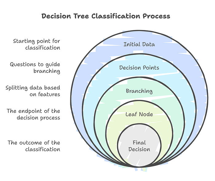
Figure 5, illustrates the Decision Tree Classification Process, breaking it into clear stages. Starting with the initial dataset, it visually represents how questions guide branching decisions based on features, splitting the data into subsets at each decision point. The process continues until it reaches the leaf nodes, which represent the endpoint of the classification, and ultimately provides the final decision. This figure emphasizes the structured and hierarchical nature of decision-making in Decision Trees, making it easier to understand their logical flow.

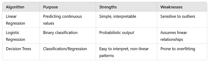
3. Comparison of Algorithms

4. Common Pitfalls and Best Practices

Pitfalls:

• Using the wrong algorithm for the task.
• Overfitting, especially with Decision Trees.
• Ignoring data preprocessing, which can degrade performance.

Best Practices:

• Perform cross-validation to evaluate model performance.
• Regularize Logistic Regression to avoid overfitting.
• Prune Decision Trees or use ensemble methods like Random Forests.

Conclusion

In this blog, we explored three essential supervised learning algorithms:

1. Linear Regression for predicting continuous outcomes.
2. Logistic Regression for binary classification.
3. Decision Trees for classification and regression.

We also discussed their strengths, weaknesses, and practical implementations in Python. In the next blog, we’ll dive into Unsupervised Learning Algorithms, focusing on clustering techniques like K-Means and Hierarchical Clustering.