Dimensionality Reduction in Machine Learning — Simplifying Complex Data for Better Insights

5 min readDec 21, 2024

Introduction

Welcome to the seventh blog in our Machine Learning Series for Beginners! 🎉

In previous blogs, we explored supervised learning, ensemble methods, and model evaluation techniques. However, real-world datasets often contain too many features (dimensions), which can make training models harder.

High-dimensional datasets are problematic because they:

Increase computational costs.
Make models prone to overfitting.
Introduce noise and redundancy, which can mislead results.
Make visualization impossible beyond three dimensions.

To solve this, we use Dimensionality Reduction techniques, which simplify data without losing critical information.

Why dimensionality reduction is important.
Popular techniques like Principal Component Analysis (PCA) and t-SNE.
Hands-on Python examples to illustrate these methods.
Real-world applications to help you understand when to use dimensionality reduction.

By the end, you’ll know how to handle large datasets effectively and make them machine learning-ready. 🚀

1. What is Dimensionality Reduction?

Dimensionality reduction is the process of reducing the number of features (dimensions) in a dataset while retaining its essential information.

It transforms the data into a lower-dimensional space.
The goal is to remove redundant or irrelevant features that do not add value to the prediction.

Analogy: Packing for a Trip 🎒

Imagine you’re going on a 3-day trip. You have a suitcase filled with 20 items — shirts, shoes, gadgets, etc. But do you really need all 20 items? Probably not.

By selecting the most essential items (like clothes and toiletries), you can reduce the weight of your luggage without compromising on your needs.

Similarly, dimensionality reduction keeps the most important features in a dataset and discards the less useful ones.

2. Why is Dimensionality Reduction Important?

Dimensionality reduction offers several benefits:

Reduces Overfitting: Models trained on fewer, meaningful features generalize better to unseen data.
Improves Training Speed: Smaller datasets require less time and computation.
Enhances Visualization: Data with many features can be visualized in 2D or 3D after reduction.
Handles Redundancy: Removes irrelevant or correlated features.

3. Types of Dimensionality Reduction Techniques

There are two main types:

Feature Selection

Selects a subset of the original features.
Examples: Removing low-variance features, Recursive Feature Elimination, and Correlation Filtering.

2. Feature Extraction

Transforms features into new combinations (dimensions).
Examples: Principal Component Analysis (PCA) and t-SNE.

We’ll focus on PCA and t-SNE because they are widely used and beginner-friendly.

4. Principal Component Analysis (PCA)

What is PCA?
PCA is a linear dimensionality reduction technique that identifies the directions (principal components) with the maximum variance in the data. It projects the data onto these components, reducing dimensions while retaining important information.

How PCA Works: Steps

Standardize the data to have a mean of 0 and variance of 1.
Compute the Covariance Matrix to identify feature relationships.
Calculate the Eigenvectors and Eigenvalues of the covariance matrix.
Sort the eigenvectors by eigenvalues (largest first) and project the data onto the top k components.

**Figure 1: Step-by-step approach to** **Achieving Dimensionality Reduction**

Figure 1 illustrates the step-by-step approach to Achieving Dimensionality Reduction. Starting with the importance and understanding of reducing dimensions, it progresses through an overview of techniques, feature selection, and feature extraction, leading to a detailed introduction and the process of Principal Component Analysis (PCA). This staircase-like structure emphasizes a logical progression, making it clear how each step contributes to simplifying complex data for better machine learning performance.

Python Example: PCA on Iris Dataset

We’ll reduce the dimensions of the Iris dataset from 4 features to 2 features for easy visualization.

from sklearn.decomposition import PCA
from sklearn.datasets import load_iris
import matplotlib.pyplot as plt

# Load the dataset
data = load_iris()
X, y = data.data, data.target

# Apply PCA
pca = PCA(n_components=2)
X_pca = pca.fit_transform(X)

# Visualize the data in 2D
plt.figure(figsize=(8, 6))
plt.scatter(X_pca[:, 0], X_pca[:, 1], c=y, cmap='viridis', edgecolor='k')
plt.xlabel('Principal Component 1')
plt.ylabel('Principal Component 2')
plt.title('PCA on Iris Dataset')
plt.show()

Output: You will see a 2D scatter plot showing clusters of flowers (setosa, versicolor, virginica).

Explanation:

PCA reduced the dimensions to 2 components while capturing the maximum variance.
The clusters show patterns clearly, even though the original data had 4 dimensions.

5. t-SNE (t-Distributed Stochastic Neighbor Embedding)

What is t-SNE?
t-SNE is a non-linear dimensionality reduction technique used primarily for data visualization.

Key Idea:

It preserves the local structure of data. Points that are close together in high dimensions remain close in the reduced space.

When to Use t-SNE?

When the dataset has non-linear relationships.
When you need to visualize clusters in complex data.

Python Example: t-SNE on Digits Dataset

Let’s visualize the Digits dataset using t-SNE.

from sklearn.manifold import TSNE
from sklearn.datasets import load_digits
import matplotlib.pyplot as plt

# Load the dataset
digits = load_digits()
X, y = digits.data, digits.target

# Apply t-SNE
tsne = TSNE(n_components=2, random_state=42)
X_tsne = tsne.fit_transform(X)

# Visualize the data
plt.figure(figsize=(8, 6))
plt.scatter(X_tsne[:, 0], X_tsne[:, 1], c=y, cmap='tab10', edgecolor='k')
plt.colorbar()
plt.title('t-SNE Visualization of Digits Dataset')
plt.xlabel('t-SNE Component 1')
plt.ylabel('t-SNE Component 2')
plt.show()

Output: You will see a beautiful 2D plot with clusters representing different digits (0-9).

Explanation:

t-SNE projects the high-dimensional data into 2D space, preserving the relationships between similar points.
Clusters emerge, making the patterns in data easier to understand.

**Figure 2: t-SNE Dimensionality Reduction Process**

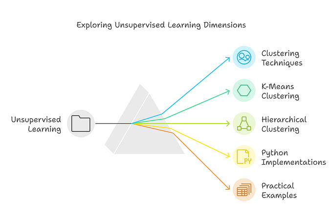
Figure 2 presents the t-SNE Dimensionality Reduction Process, breaking down the key steps involved in using this technique. It starts with data standardization and moves through calculating and sorting eigenvectors and eigenvalues, projecting data onto components, and transitioning to an overview of t-SNE. The figure highlights t-SNE’s ability to preserve local structure in data and showcases its use cases for non-linear dimensionality reduction and data visualization. The spiral design emphasizes the iterative and explorative nature of t-SNE.

7. Real-World Applications of Dimensionality Reduction

Image Processing

Reduce image resolution or pixels to speed up computations.

2. Text Data Analysis

Simplify TF-IDF or word embeddings (Word2Vec, GloVe) for NLP tasks.

3. Genomics and Bioinformatics

Analyze gene expression data by reducing redundant features.

4. Customer Segmentation

Simplify datasets for clustering customer behaviors and preferences.

5. Recommendation Systems

Reduce dimensions in user-item interaction matrices.

8. Key Takeaways

Dimensionality Reduction helps simplify high-dimensional datasets without losing essential information.
PCA is a linear technique that reduces variance while keeping the data interpretable.
t-SNE is a powerful non-linear technique, great for visualizing complex datasets.
These methods improve model performance, reduce overfitting, and enable better data visualization.

Conclusion

In this blog, we explored Dimensionality Reduction techniques like PCA and t-SNE. Both methods help simplify data and make machine learning models faster, more accurate, and easier to interpret.

What’s Next?
In the next blog, we’ll explore Clustering Algorithms like K-Means and Hierarchical Clustering — key methods for grouping data in unsupervised learning.